1. Create a project

Add State layers

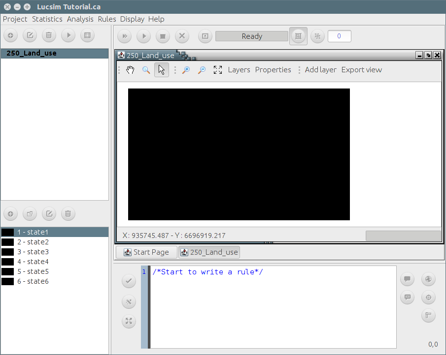
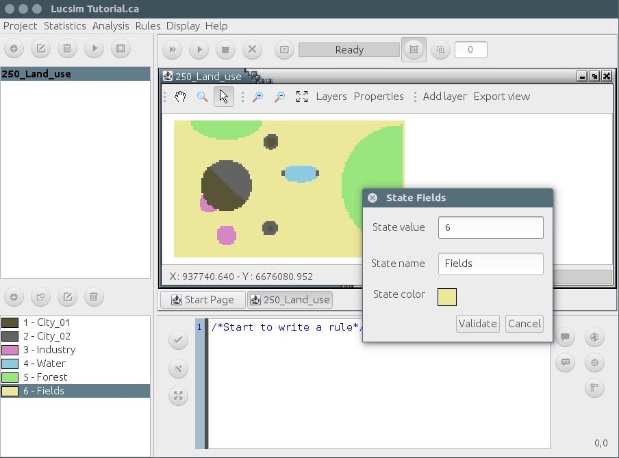
State layers are TIF images where pixels codes correspond to CA states (in LucSim, these states should correspond to land use categories or assimilated classes). They can be added to the project by clicking on the “Add” button from the "Layers" windows. When states are opened in LucSim, all land use categories contained in the original TIF image are listed in the "State" Window, and appear black-colored with no name (only a number). Colors and names can be changed by double clicking on the state name or using the “Modify State” button. User can add as many state layers as he needs by clicking an the “Add layer to the list” button and answering "Yes" to the automatic question “Is is a State layer ?”. These layers are the basical data needed to run CA simulations.

Exercise
1. Open Land use 1 and Land use 2
2. Modify states name and color
3. Switch from one layer to another
4. Save your project

Add other layers

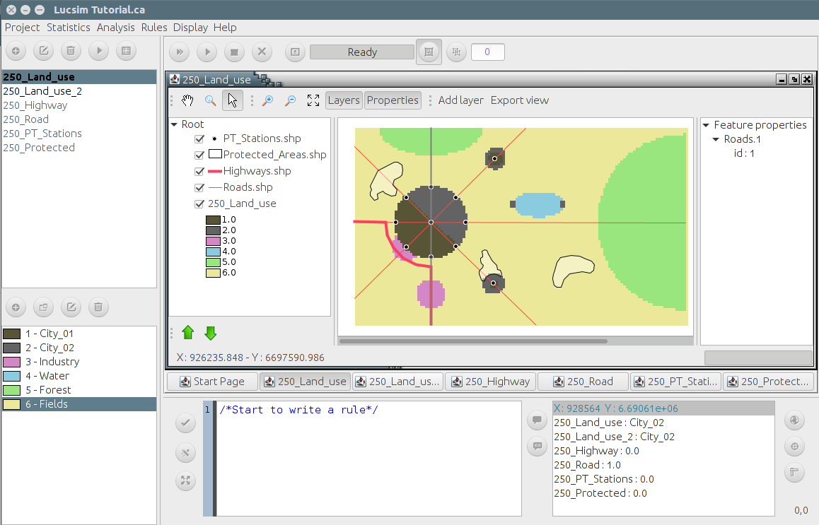
Other layers are TIF images that do not contain CA states but other kind of information like routes, public transport stations or protected areas. When adding this kind of layers to the project, user should answer “no” to the question “Is is a State layer ?” (“Add layer to the list” button). Layers’colors can be modified in the "Maps" windows by clicking on the button “Layers”. On the left, this button displays on new frame showing the modifiable key of the layers. Notice that these layers can be used to calculate models results and/or to calibrate CA transitions rules, but not to run CA simulations.

Exercise
1. Add routes, highway, Stations and protected areas to the project (TIF)
2. Display and modify the key in the left frame of the "Maps" window
3. Zoom in, zoom out and display a full view of the layers

Display additional shapefiles

Shapefiles can be added to display additional geo-information on the layers of the project. To add shapefiles, click “Add layer” from the "Maps" window. The key of the layers can be accessed and modified on the left frame ("Layers" button): change single symbol, foreground and background colors, line width and layer's opacity. Notice that shapefiles are only used to display information, not to calculate anything within the models implemented in LucSim.

2. Statistics

Display graph

For each layer a graph can be display from the menu "Display" (check box). This graph summarizes the number of cells bu land uses for state layers in different ways (pie chart, histogram) and colors (colors are predefined or defined by the user ; see section 1.1). On the bottom of the box, a table also indicates the number and the percents of cells in each category. Notice that “Curve” and “Step” options are only available if a CA simulation was previously launched (see section 4.2).

Layer comparison

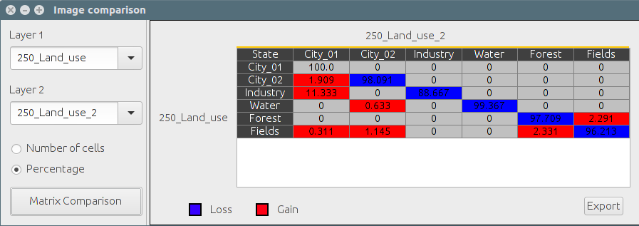
To compare the states (land uses) of two images, use the "Image comparison" option from the "Statistics" menu. The name of the two images to be compared must be chosen in the dropdown list on the left on the dialog box, and user must indicate if the results are calculated in percent or in number of cells. Clicking on the “Matrix calculation” button will process the calculation. The results are automatically displayed on a matrix on the right. Blue cells of the matrix correspond the a loss between the first and the second image. Red cells correspond to a gain.

Exercise
1. Calculate "Image comparison" between Land Use 1 and Land Use 2
2. Switch from percents to numbers of cells
3. Export the results in CSV format and open it in spreadsheet

Neighborhood extraction

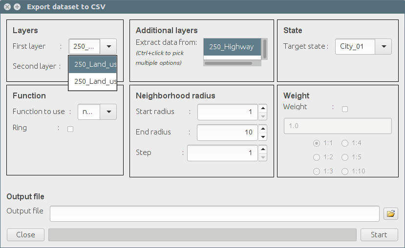
For further and more complex statistical analysis, the spatial neighborhood and land uses (for all or for specific cells) can be extracted from LucSim and used as an input for statistics dedicated softwares. To extract a neighborhood, use the option “Neighborhood extraction" from the "Statistics" menu. This tool aimed to help the user get insight from the neighborhood surrounding cells that underwent a specific transition. From left to right and from top to bottom, the dialog box asks for (1) the first and second layers data must be extracted from (the neighbourhood from the first layer will be extracted, the state from the second layer helps to locate cells that underwent the transition the user can be interested about), (2) additional non state layer to be included in the extraction results, (3) Target state of the neighborhood (e.g. neighborhood of the “City” cells (target) will indicate in a dedicated column whether or not the cell made a transition toward “City”), (4) Neighborhood function allowing to choose between square, circle or ring neighborhood, (5) Neighborhood radius demanding starting distance (in pixel), ending distance and number of steps, and (5) optional weighting. Extracted neighborhood must then be saved in an output CVS file.

3. Analysis

Markov chains

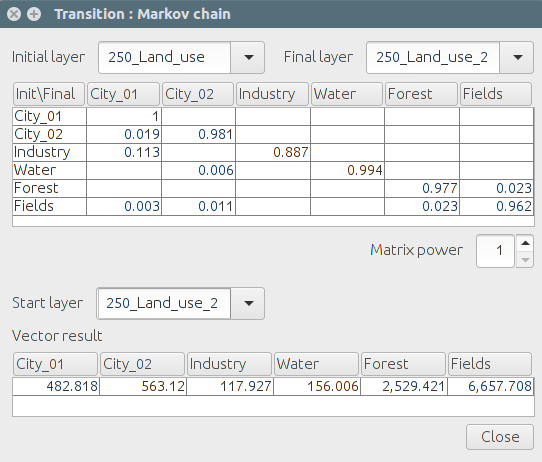
Markov chains are a mean to calibrate CA simulations in time: CA simulation stops when the number of cells of one or several states predicted by the markovian process is reached (for further explanations about the model, please refer to the LucSim complete documentation). To use this function, a Markov chain must be calculated via the “Analysis” menu. In the dialog box, a transition matrix is automatically computed when “initial” and “final” layers are chosen. This matrix contains the probability of transition (for a land use cell) from a state to another state (a null probability means that the transition is impossible) in one simulation step, as observed between the initial and final layers. “Matrix power” is an option that modifies the probabilities of transition for simulating more than one step (Power 2 corresponds to 2 steps, Power 3 to 3 steps and so on). Finally, these probabilities of transition can be applied to a layer in order to simulate land use changes in the future (vector result from t+1 to t+n according to the matrix power). Results are automatically saved in LucSim. Markov chains when only be taken into account when the markovian constraints are applied in the CA simulation (see section 4.4).

Exercise
1. Calculate the transition matrix between Land Use 1 and Land Use 2 and analyze the results
2. Apply these probabilities to Land Use 2 and visualize Land Use 3 (vector result)
3. Apply a Matrix Power 2 to land Use 2 and visualize Land Use 4
4. Copy and paste the results (transition matrix and vector result) in a spreadsheet
5. Close the box, results are saved

Potential model

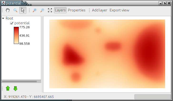
The potential model allows to analyze the possibilities of expansion of a land use according to the concepts of spatial interaction (for further explanations about the model, please refer to the LucSim complete documentation). The calculation of a potential is done from the “Analysis” menu. The dialog box asks to define: (1) the layer used to perform the calculation, (2) a “mass” of attractiveness for each land use category (e.g. from 0 to 10), (3) the exponent of the distance (optional), (4) the size of the neighborhood for the calculation, and (5) a name for the “Result layer”. Click on “Create” to compute the results. Resulting layer is automatically displayed in a new tab of the “Maps” window and its key can be analyzed and modified using the “Layers” button of the same window.

4. Transition rules and simulation

Rules edition

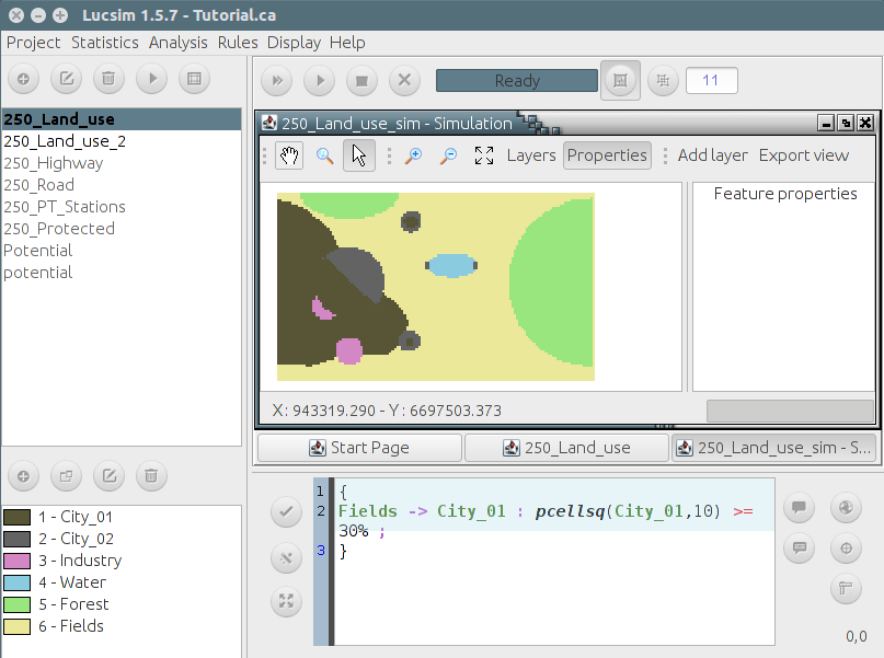
LucSim transition rules must be written in the “Rules editor” (displayed via the “Display” menu). Rules edition is based on a complex syntax specifically designed for LucSim. Basically, this syntax demands to define (1) a departure state and an arrival state separated by (->) and followed by (:), (2) a transition function associated with two parameters (a land use and a distance in pixels), (3) a condition expressed in land use percents or number of cells and (4) a semicolon (;) ending the rule. Several rules can be combined with logical operators (and, or, etc.). Rules can be grouped together using braces ({}) to manage their occurrences and priority. For further explanations about LucSim rules edition, please refer to the complete documentation. When rules are edited, they can be launched using the “Simulation bar” (see section 4.2).

Exercise
1. Imagine that fields become city if surrounded by 30% of city within 10 pixels
2. Use the corresponding rule : Fields -> City_01 : pcellsq(City_01,10) >= 30% ;
3. Test the validity of the rule (button)
4. Launch the simulation and observe the results
5. If something happened, take a beer, you are a champion !

Simulation bar

Simulation bar can intuitively be used like a MP3 player to launch the simulation (in continue or step by step) and to stop or reset the simulation. When a simulation runs, a progress bar indicates the evolution of the simulation at each step and a counter is incremented on the left. From the simulation bar, user can choose between synchrone (by default) and asynchrone simulation mode. Simulation stops when CA reaches the final step (indicated in the counter).

Exercise
1. Step by step, launch three simulation steps , observe the “Map” and reset when finished
2. Launch the simulation in continue and observe the final step in the counter
3. Launch the same simulation in asynchrone mode and observe the difference
4. Export a view of the final step in PNG or SVG format